Using the Spreadsheet Study

Related Documentation

• Overview of Spreadsheet Studies
• Using the Spreadsheet Study
• Spreadsheet Systems, Alerts and Automated Trading
• Spreadsheet Study Inputs
• Referencing Other Charts in Spreadsheet Study Formulas
• Spreadsheet Studies Special Tasks
• Sharing Your Spreadsheet Study With Another User
• Working with Spreadsheets
• Spreadsheet Functions
• Spreadsheet Example Formulas and Usage

On This Page

• Step By Step Instructions to use the Spreadsheet Study
• Clearing Old Study and Other Data from Spreadsheets
• Automatic Hiding of Spreadsheet Windows
• Decimal Point and Function Parameter Delimiters
• Order of Study Data Outputted to Spreadsheet
• Imprecision of Floating-Point Numbers and Comparisons
• Rounding of Values to Tick Size
• Using a Formula in Formula Columns Row 2
• Preventing Effect of Changes to Study Order and Subgraphs Outputted on Formula References to Study Subgraphs
• Solving Study Not Displaying on Spreadsheet Sheet

Step By Step Instructions to use the Spreadsheet Study

1. Go to an open chart or open a chart.
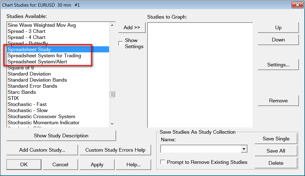
2. Select Analysis >> Studies on the menu.'
3. Select Spreadsheet Study Studies Available list. Press the Add button. If you want to create a System or Alert, then you will need to add the Spreadsheet System/Alert study instead. For more information about Systems and Alerts, refer to the Spreadsheet Systems and Alerts page.
   
4. Highlight Spreadsheet Study or Spreadsheet System/Alert in the Studies to Graph list. Press the Settings button.
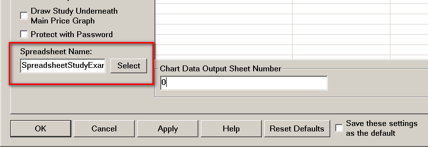
5. In the Study Settings window on the Settings and Inputs tab, there is a text box for the Spreadsheet Name. Enter a name in the text box without an extension (refer to image below). This is the name of the Spreadsheet that will be opened or created, to contain the data and formulas. The name should be related to what your custom study will do. For example, you can enter MovingAverage to indicate it is for a moving average. If there is no Spreadsheet with this name already, then a new Spreadsheet will be created. The Spreadsheet will be automatically opened or a new one will be created.
   
6. If you want to use a Spreadsheet you created before and previously saved, then press the Select button beside the Spreadsheet Name box and select it.
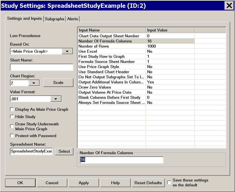
7. On the Settings and Inputs tab, set the the Inputs and other settings as you require. For a description of the available Inputs for the Spreadsheet Study study, refer to Spreadsheet Inputs for general Inputs, and Spreadsheet Study Inputs that are Specific to Systems, Alerts, and Automated Trading for Inputs specific to Systems and Alerts. Spreadsheet Inputs for Systems and Alerts only apply when using the Spreadsheet System/Alert study.
   
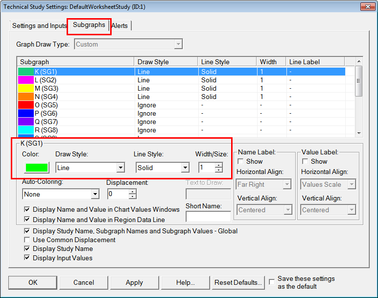
8. Select the Subgraphs tab. Adjust the settings for each Subgraph as you require. Each Subgraph corresponds to a formula column on the Spreadsheet. If you want a formula column to be visible on the chart, then set its Draw Style to something other than Ignore or Hidden. For example, use a Draw Style of Line . Otherwise, set the Draw Style to Ignore.
   
9. Coloring Bars Based on Certain Conditions: If you wish to create a study which colors bars based upon a certain condition, then you will want to set the Draw Style for the Subgraphs you will be using to Color Bar. If you wish to color bars just one color, then you will just need only one Subgraph and the Draw Style for the others should be set to Ignore. If you wish to color the bars 2 colors, then you will need 2 formula columns and you will want to set the Draw Style for 2 Subgraphs to Color Bar and set the Subgraphs to the colors you want. Keep in mind for a Color Bar Spreadsheet study, you must be using the Spreadsheet Study study. You can also color bars by using the Color Bar Based on Alert Condition study.
10. Press the OK button to close the Study Settings window for the Spreadsheet study.
11. If there are other studies you want to add to the chart that have not already been added or studies you want to reference in the Spreadsheet formulas, then add them now and adjust the settings as you require them for each study. Simply select them from the Studies Available list or through Add Custom Study and press the Add button.
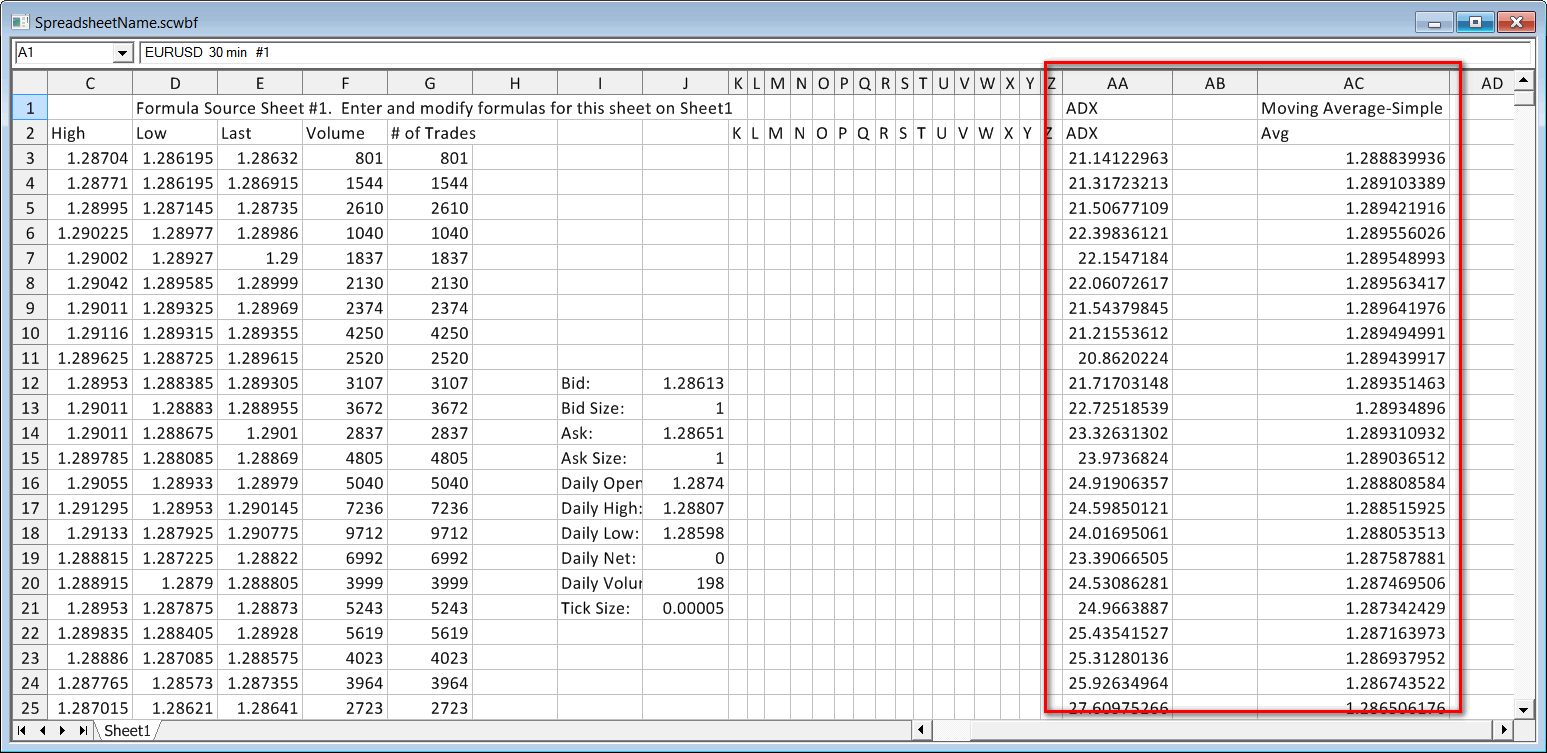
12. These studies will be outputted beginning at column AA on the Spreadsheet, by default. If the Number of Formula Columns Input is set to a number greater than 16, then the studies will be outputted to a column higher than AA.
    
13. If you wish to have access to Bid Volume and Ask Volume, then add the Bid Volume and Ask Volume studies to the chart as well.
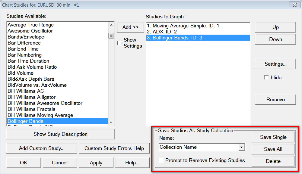
14. The order in which studies are outputted beginning at column AA on the Spreadsheet depends upon the order they are listed in Studies to Graph.
15. It is strongly recommended when referencing the data from Study Subgraphs in the Study columns to use the New Spreadsheets referencing method for Study Subgraphs. The reason this is recommended is because if some studies are reordered or removed, then the particular Sheet columns they are outputted can change which will affect traditional cell reference methods. However, with this new referencing method which refers to the Study by its own ID and Subgraph, there is no effect if a particular Study moves in relation to the Sheet columns.
16. If you added a study to the chart for the purpose of only referencing it in your Spreadsheet formulas and do not want to make it visible on the chart, then in the Study Settings for the study enable Hide Study.
17. Type a name that you want to save your Spreadsheet Study as into the Save Studies As Study Collection >> Name text box. You can also select an existing name from the drop-down list. This name can be the same as the Spreadsheet Name you entered earlier, or a similar name. It does not have to match.
    
18. In order for the use of Study Collections to work properly with the Spreadsheet studies, the Chart Data Output Sheet Number Input with the Spreadsheet Study needs to be set to 0.
19. Press the Save Single button or Save All button. If your Spreadsheet formulas will use the results of other studies on the chart, then you must press the Save All button when saving the Study Collection. For more information, refer to Study Collections.
20. Using a Study Collection will let you apply your Spreadsheet Study or Spreadsheet System/Alert and all the settings, to the chart or any other chart with a single step by selecting the Study Collection name from the Sierra Chart Analysis menu.
21. If you apply the Study Collection to multiple charts, they will use the same Spreadsheet file. Each chart will use a separate Sheet# within the Spreadsheet. Chart #1 will use Sheet1, chart #2 will use Sheet2 and so on.
22. Press the OK button on the Chart Studies window.
23. The Spreadsheet window will be opened in the background. Go to it by selecting CW >> [Spreadsheet Name] on the menu. The name will be what you have entered in a prior step plus a .scss extension.
    
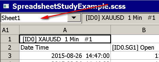
24. A Spreadsheet contains multiple Sheets. The Sheet number (Sheet#) the chart data is outputted to, is the same number as the Chart Number. For example, Chart #2 will be outputted to Sheet2 in the Spreadsheet. This is a very important functional item to understand.
25. The Sheets are selected with a list box at the top left of the Spreadsheet window. Refer to the image below.
    
26. All of the individual studies on the chart are also outputted to the same Sheet# beginning at column AAby default. The starting column can be further to the right if the Number of Formula Columns Input is set to a number higher than 16. For example, if the Number of Formula Columns is 17, the studies will start at AB.
27. It is possible to output chart data to a different Sheet# that differs from the Chart Number. By default chart data is outputted to the Sheet# with the same number as the Chart Number when the Chart Data Output Sheet Number Input with the Spreadsheet study is set to 0. However, if this is set to a different number, then chart data will be outputted to the Sheet# which corresponds to the Chart Data Output Sheet Number Input.
28. If you were to rename the Sheet# that the chart data is outputted to with Spreadsheet >> Rename, then what will happen is that a new Sheet will be inserted with the name Sheet# where # is equal to the Chart Number or the Chart Data Output Sheet Number if it is not set to zero.
29. If the Sheet# in the Spreadsheet window has been previously used by the Spreadsheet Study, then whatever data that was previously outputted, saved, and not overwritten with the current data in the chart will still be there. You will have to manually delete that data if you want. Simply highlight the cells you want to delete and press the Delete key on the keyboard.
30. The Date and Time of each chart bar are outputted to column A. The rest of the chart bar values are placed in the subsequent columns.
31. You will be entering your formulas in columns K through Z on the Sheet. More formula columns are available by setting the Number of Formula Columns Input to a higher number.
32. Formulas must go in row 3 and not any other row. By default, only the first 4 Spreadsheet Study formula columns are graphed on the chart (K, L, M, N). The remaining columns (M through Z, assuming the default of 16 formula columns) can be optionally graphed as well. To graph these columns on the chart, go to the Study Settings window for the Spreadsheet Study on the chart and set Draw Style to the desired style for the corresponding Subgraph.
    
33. The Draw Style for the K, L, M, N Subgraphs can be set to Ignore to not graph them on the chart. Any spreadsheet column that is not graphed can be used for background calculations required for your analysis method.
34. A Spreadsheet file contains multiple Sheets, each named Sheet#. The Sheet you must enter your formulas on might be different than the Sheet the chart data is copied to. Be sure to refer to the Formula Source Sheet Number Input description for clarification on this.
35. By default, when you add the Spreadsheet Study to a chart, then the Sheet # the chart data is copied to, are where the formulas need to be entered unless the Spreadsheet Study was applied to the chart as part of an existing Study Collection. In this case the Sheet# for your formulas may be different.
36. The chart data is outputted to the Spreadsheet beginning at row 3. Your formulas must be entered in row 3 when entering the formulas in the Spreadsheet Study formula columns K through Z.
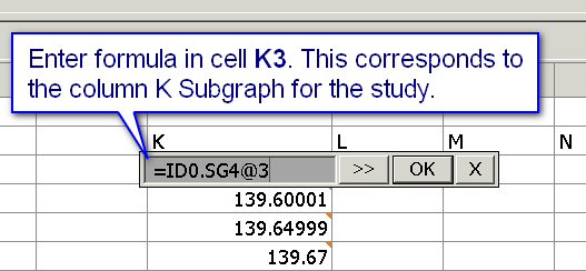
37. The Number of Rows Input in the Study Settings window sets the number of rows the formula is copied down to. For example: if you enter =ID0.SG4@3 + 2 in K3 and the Number of Rows study Input is set to 1000, then it will be copied all the way down to K1002. The reference to ID0.SG4@3 will automatically be adjusted for each row.
38. For an understanding of references like ID0.SG4@3, refer to References to Study Subgraph Columns when using the Spreadsheet Study. In this case, this refers to the main price graph and the fourth Subgraph, which is the last trade price. It is essential that you use this method of referencing study Subgraphs.
39. If you need more formula columns, then you can increase the Number of Formula Columns Input with the Spreadsheet Study.
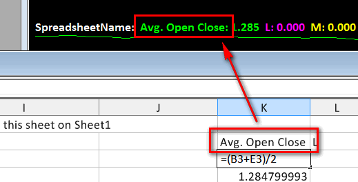
40. Example Formula: To create a five bar moving average of closing prices on the chart: Enter: =AVERAGE(ID0.SG4@3:ID0.SG4@7) in cell K3. Referred to the image below. For instructions to enter the formula, refer to Entering Data.
    
    The range ID0.SG4@3:ID0.SG4@7 is the last 5 closing prices from the chart.
    
41. For the formula to automatically fill down the formula column and for the chart to automatically update, it is necessary that Global Settings >> Spreadsheet Settings >> Spreadsheet Study >> Recalculate the Chart When a Formula Column is Changed option be enabled. If it is not, go to the chart as explained in the next step, and select Chart >> Recalculate.
42. To see the result of this formula on the chart select the chart from the CW menu.
43. The moving average will be drawn in Chart Region 2. To put it in Chart Region 1 over the price bars, go to chart window. Select Analysis >> Studies on the menu. Select the name of your Spreadsheet in the Studies to Graph list box (the Spreadsheet Study will have been renamed to the Spreadsheet name). Press the Settings button. Set the Chart Region setting to number 1. Press OK. Press OK.
44. The formula example given above is very simple. You can use formulas to perform most any kind of calculation that you require. Refer to the Working with Spreadsheets documentation page for complete information on using Spreadsheets, creating and entering formulas, and the available Spreadsheet Functions to use in formulas.
45. Color Bar Formula Example: If you are creating a Spreadsheet Study to color bars based on certain conditions, then your formula should return TRUE or FALSE. For example if you wish to color bars that have a Last Price above 100, then you would use this formula: =ID0.SG4@3>100.
    
    In the case of coloring bars with one color based on a single formula, you probably would just simply want to use our Color Bar Based on Alert Condition study which will color bars based on the specified Alert Condition using similar formulas.
46. You are able to reference studies in the chart that contains the Spreadsheet Study, in the Spreadsheet formulas. Remember that all of the studies on the chart are outputted beginning at column AA on the corresponding Sheet#.
    
    They can be outputted beginning at a more rightmost Column, if the Number of Formula Columns Spreadsheet Study Input is set to a number higher than 16. The order in which studies are outputted beginning at column AA depends upon the order they are listed in the Studies to Graph list on the Chart Studies window.
47. If your formula returns a value of zero, then the zero value will not be drawn in the study graph on the chart unless you set the Draw Zeros Input with the Spreadsheet Study to Yes.
48. When entering numbers and formulas, keep in mind to use the proper delimiters in the numbers for the decimal point and between the function parameters for formulas. Refer to Decimal Point and Function Parameter Delimiters.
49. The Spreadsheet will need to be saved when you close the Spreadsheet or Sierra Chart, so you do not lose any of your formulas. First, go to the Spreadsheet window. Select File >> Save on the menu to save the Spreadsheet. You will also be asked to save changes when you close Sierra Chart or the Spreadsheet.
50. Enter a custom name for any of the available formula columns that you use. To name column K, type the name in cell K2. These names will be displayed as the Subgraph names for the study graph in the chart.
    
51. Click on the links to download the Study Collection and Spreadsheet files that demonstrate exactly the example we have given in the step-by-step instructions here. These files need to be saved to your Data Files Folder. You can find the location of this folder under Global Settings >> General Settings.

Clearing Old Study and Other Data from Spreadsheets

It is a good idea to clear any remaining data in the cells of the Sheets in a Spreadsheet which are no longer being used. This improves overall Spreadsheet performance and reduces the amount of time to save a Spreadsheet.

To reduce the number of rows used in a Sheet which are being used by the Spreadsheet Study, reduce the Number of Rows Spreadsheet Study Input. When you reduce this Input, the unused rows will automatically be cleared from the Sheet. You can verify this and delete any rows which might remain.

When using one of the Spreadsheet studies on a chart, and you have added other studies to the chart, then when you remove those other studies from the chart, there may be still some study data displayed from the prior studies which have been removed, beginning at column AA on the Sheet being used by the Spreadsheet study in the Spreadsheet.

Follow the steps below to remove any old and unused to data in a Sheet.

1. Go to column AA in the corresponding Sheet in the Spreadsheet window that is linked with the Spreadsheet Study you are using.
2. Select all of the columns beginning with column AA that contain data for studies that are no longer on the chart. You can select the column by left clicking on the column header with the Pointer. While holding the left pointer button, you can drag it towards the right to select additional columns.
3. Press the Delete key on the keyboard to delete the data.

Automatic Hiding of Spreadsheet Windows

A Spreadsheet window that is being referenced by a Spreadsheet study on a chart that is not visible because the chart is in a chartbook which is not currently visible, will be hidden. However, there is a way around this and allow the Spreadsheet window to always be visible. in the currently visible chartbook, at the Spreadsheet study to a chart and have it reference the same Spreadsheet name. In the Spreadsheet study you may want to set the Chart Data Output Sheet Number Input to an unused Sheet in the Spreadsheet window, to prevent overwriting the information from the chart that is also using it in another chartbook.

Decimal Point and Function Parameter Delimiters

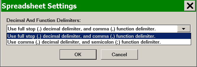
When entering Spreadsheet formulas, it is necessary to use the correct decimal point and function parameter delimiter that corresponds to the setting in Global Settings >> Spreadsheet Settings >> Decimal and Function Delimiters . Refer to the image below.

When changing this setting, existing formulas on the Spreadsheets are changed to use the selected delimiters.

Order of Study Data Outputted to Spreadsheet

The data for all studies on a chart are outputted to the Sheet in the Spreadsheet being used by the Spreadsheet study on a chart. The default column this begins at is column AA but could be a later column depending upon the Number of Formula Columns Input setting for the Spreadsheet Study.

The data for each study Subgraph with a name is outputted to the Sheet unless the Draw Style is set to Ignore and Do Not Output Subgraphs set to Ignore is set to Yes.

The order that the study Subgraphs are outputted to the Sheet is the order in which the studies are listed in the Studies to Graph list in the Analysis >> Studies window. Adding, removing, or reordering studies changes the position of the studies outputted to the Sheet. For this reason, it is important to use New Spreadsheets and reference Study Subgraphs using the References to Study Subgraph Columns when using the Spreadsheet Study method.

There is a blank column between each study outputted to the Sheet.

When using the Study/Price Overlay study, it is possible when opening a Chartbook, that the number of Subgraphs it contains will change because the study it is referencing may not be loaded when its data is outputted to a Sheet. This has the effect of causing the outputted study data to shift causing data to be outputted to Sheet columns which later are not being used when the charts are all loaded in the Chartbook. This can cause confusion.

In this particular case described above, what you need to do is select the column headers where the study data is outputted to highlight the columns containing the study data. Press the Delete key on the keyboard to delete the data. Go to the chart that contains the Spreadsheet Study referencing that particular Sheet that you deleted study data from and select Chart >> Recalculate. This process will clear data from all columns which are not actually being used to make it clear which columns are being used.

Imprecision of Floating-Point Numbers and Comparisons

Floating point numbers, numbers with digits after the right side of the decimal point, in Sierra Chart are stored in most cases as 4 byte single precision floating point numbers. Main price graph and study graph data are stored as 4 byte single precision floating point numbers.

When these numbers are outputted to Sheets in Spreadsheets, these numbers are also stored as floating-point numbers.

It is important to understand what is known as floating point error. Refer to Accuracy Problems in the Floating Point Wikipedia article. For example, the number .01 may internally be represented in a single precision floating-point variable as .0099998.

Formulas which perform calculations on numbers, very likely also will have floating-point error in the result even though you may not visually see it.

To visually correct this accuracy problem, select a cell or a column of cells containing the numbers in a Sheet and select Spreadsheet >> Number Format on the menu. Choose the appropriate Number Format you want to use to format the numbers as you require and hide the effect of this accuracy problem.

The above also applies to the display of the study values on the chart. To visually correct this accuracy problem, change the Value Format setting for the study to format the numbers as you require and hide the effect of this accuracy problem.

Spreadsheet formulas will always work with the unformatted numbers. These numbers can be imprecise even when referencing cells that have an applied Number Format.

The Number Format has no effect upon the internal calculations. For example, the number .01 may internally be represented as .0099998. So it becomes necessary to consider this when writing a formula. For example if you want to determine if .0099998 and .0100001 are equal, the formula should be written as =ABS(.0099998 - .0100001) < .005. A similar kind of technique can be used for other kinds of comparisons.

When using the Formula Expression Tree, the precision of the displayed numbers is not necessarily the actual full precision. There could be additional decimal places of precision beyond 6 places which are not displayed. This is something to keep in mind.

Rounding of Values to Tick Size

Use the following Spreadsheet formula to round a value to the Tick Size.

=MROUND([cell reference],$J$21).

If the Tick Size value that is displayed in cell J21 shows floating point rounding errors itself, then it is necessary to use two cells to perform the rounding to the nearest tick size. A floating point error is due to how computers handle floating point variables (numbers with decimal places), in which you may see something like .2500011, instead of just 0.25. To clean up the Tick Size values when they are less than 1.0 and then perform a final adjustment based on the corrected Tick Size, follow these instructions:

• In cell H21, enter the following: =1/ROUND(1/J21, 0).
• Use the following formula in an appropriate cell to round a value to the nearest Tick Size: =MROUND([cell reference], $H$21).

Using a Formula in Formula Columns Row 2

Just as you can enter a custom name for any of the available formula columns that you use, as described in the Step-by-Step Instructions, you can also use a formula to generate the name.

In the same way as you enter a name for column K, you can instead type a formula for the name in cell K2. The result of the formula will be displayed in the cell as well as the Subgraph name for the study graph in the chart.

For this to work, the formula must result in a text value. If the result of the formula is not a text value, but a number, error, empty value, or something else, the formula will be replaced with the default name of the column. The spreadsheet formula function TEXT may be used to convert numbers to text values, if necessary.

For example, if you are using cell K1 to store information used by your formulas that is also relevant to the name of the column, you could use that value as part of the name. You can do this by using one of two following formulas depending on whether the data in cell K1 is a number or is text:

• Data in K1 is a number: K2: = TEXT(VALUE(K1)) + " Bar Average"
• Data in K1 is text: K2: = K1 + " Bar Average"

So if the value in K1 is 10, the name for the formula column and Subgraph will be 10 Bar Average.

The Subgraph name in the chart may not update right away, but you can manually update the chart by selecting Chart >> Recalculate from the menu.

Preventing Effect of Changes to Study Order and Subgraphs Outputted on Formula References to Study Subgraphs

When using one of the Spreadsheet Studies, and the formulas are referencing study Subgraph values which begin at column AA (assuming Number of Formula Columns is set to 16), then as the studies are reordered on the chart, added or removed, or there are a different number of Subgraphs outputted to the Sheet by a particular study, this will affect formula references if using the A1 referencing method.

The proper solution to this is to reference study Subgraph cells using the References to Study Subgraph Columns when using the Spreadsheet Study method. This is absolutely essential. You should never reference study Subgraphs by using the A1 reference notation. One day you will regret this if you do.

Additionally there are the following Spreadsheet Study Inputs and Study Settings for controlling the Study Subgraphs output to a Sheet:

1. Do Not Output Subgraphs Set To Ignore Input. This is useful when the Study Subgraph Draw Style is set to Ignore.
2. Include in Spreadsheet Study Setting
3. Subgraph >> Include in Spreadsheet Study Subgraph Setting

Solving Study Not Displaying On Spreadsheet Sheet

If a particular study that has been added to the chart is not displaying on the particular Sheet the chart data is being outputted to in the specified Spreadsheet used by the Spreadsheet Study, then follow the instructions below.

These instructions also are applicable to when you do not want to output a particular Study or particular Study Subgraph to the Sheet used by the Spreadsheet Study.

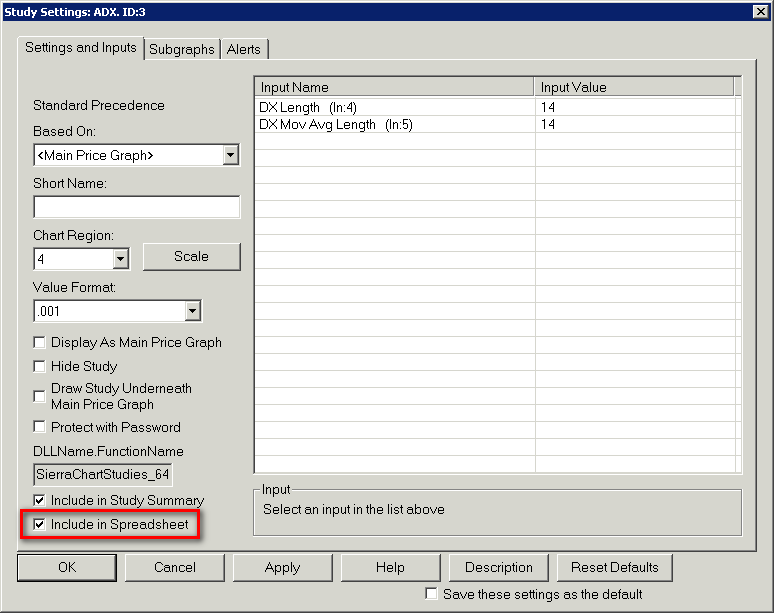
1. Open the Study Settings window for the study that is not displaying.
2. Select the Settings and Inputs tab.
3. Make sure Include in Spreadsheet is enabled as in the image below. Or disable it if you do not want the study outputted to the Sheet used by the Spreadsheet Study.
   
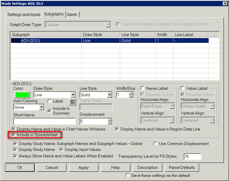
4. Select the Subgraphs tab.
5. Select a particular subgraph from the list.
6. Make sure Include in Spreadsheet is enabled as in the image below. Or disable it if you do not want the study Subgraph outputted to the Sheet used by the Spreadsheet Study.
   
7. If the spreadsheet Study Input Do not Output Subgraphs Set to Ignore is set to Yes, then make sure the Draw Style for any Subgraphs you want to see in the Spreadsheet are not set to Ignore.
8. Additionally, another reason why a Study or its Subgraphs are not outputted or not fully outputted to a Sheet is due to calculation order. This is explained in the Study Calculation Precedence section.